Working with Gridded Data#
Download this notebook: xarray_workflow.ipynb
Climate and environmental data rarely arrive as a tidy matrix. They arrive as
labelled xarray objects: a temperature field over
latitude and longitude, a covariate such as elevation, and gaps where a sensor
failed or a cloud covered the scene. A GP in GPJax, on the other hand, consumes a
Dataset of flat inputs \(\mathbf{X} \in \mathbb{R}^{N
\times D}\) and outputs \(\mathbf{y} \in \mathbb{R}^{N \times 1}\).
The gpjax.xarray module converts between the two at the
edges of a workflow. In this notebook we
flatten a gappy, labelled field into a
Datasetwithfrom_xarray,fit a GP exactly as we would on any other
Dataset,predict the mean and variance on a finer grid with
GridSpec.predict, anddraw joint posterior samples on that grid with
GridSpec.inputs_forandGridSpec.to_xarray.
For the same workflow on real data, see Infilling Global Surface Temperature.
The module needs the optional extra: pip install "gpjax[xarray]".
from jax import config
import jax.numpy as jnp
import jax.random as jr
from jaxtyping import install_import_hook
import matplotlib.pyplot as plt
import numpy as np
import xarray as xr

config.update("jax_enable_x64", True)

with install_import_hook("gpjax", "beartype.beartype"):
    import gpjax as gpx
    from gpjax.xarray import (
        Standardise,
        from_xarray,
    )

key = jr.key(42)
gpx.plotting.use_style()
'ledger'
A synthetic temperature field#
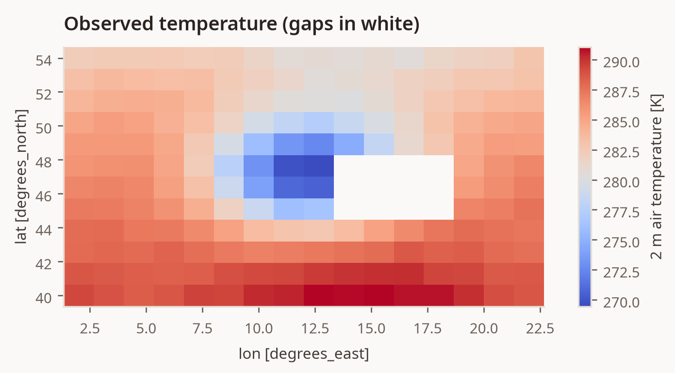
We simulate near-surface temperature on a regional latitude-longitude grid. It cools towards the pole and with elevation (a lapse rate of roughly 6.5 K per kilometre), with a smooth large-scale anomaly on top. Elevation is a separate variable over the same grid. The data are synthetic, so the notebook needs no download and every number in it can be checked against the truth.
def elevation_at(lat, lon):
    """A single mountain range, in metres."""
    return 2500.0 * np.exp(-(((lon - 12.0) / 4.0) ** 2) - ((lat - 47.0) / 3.0) ** 2)


def temperature_at(lat, lon, elevation):
    """Temperature in kelvin: latitude gradient, lapse rate and an anomaly."""
    anomaly = 1.5 * np.sin(lon / 3.0) * np.cos(lat / 4.0)
    return 290.0 - 0.6 * (lat - 40.0) - 0.0065 * elevation + anomaly


def regional_field(lats, lons) -> xr.Dataset:
    lat_grid, lon_grid = np.meshgrid(lats, lons, indexing="ij")
    elevation = elevation_at(lat_grid, lon_grid)
    return xr.Dataset(
        {
            "t2m": (
                ("lat", "lon"),
                temperature_at(lat_grid, lon_grid, elevation),
                {"units": "K", "long_name": "2 m air temperature"},
            ),
            "elevation": (("lat", "lon"), elevation, {"units": "m"}),
        },
        coords={
            "lat": ("lat", lats, {"units": "degrees_north"}),
            "lon": ("lon", lons, {"units": "degrees_east"}),
        },
    )


coarse = regional_field(np.linspace(40.0, 54.0, 12), np.linspace(2.0, 22.0, 16))
Real observations have holes. We knock out a block of cells, as a cloud would, and add a little measurement noise to the rest.
key, noise_key = jr.split(key)
noise = 0.2 * np.asarray(jr.normal(noise_key, coarse["t2m"].shape))
observed = coarse.copy(deep=True)
observed["t2m"] = observed["t2m"] + noise
observed["t2m"].attrs = coarse["t2m"].attrs
observed["t2m"][4:7, 9:13] = np.nan

observed["t2m"].plot(cmap="coolwarm")
plt.title("Observed temperature (gaps in white)")
plt.show()
From labelled data to a Dataset#
from_xarray takes the target variable and the inputs we want the GP to depend
on. Inputs can be coordinates (lat, lon) or other data variables
(elevation), and the columns of \(\mathbf{X}\) follow the order we list them in.
Cells where the target or any input is NaN are dropped by default, and the
returned GridSpec records which ones.
Temperature varies over degrees of latitude and longitude, but over hundreds of
metres of elevation. The Standardise transform
scales each input to zero mean and unit standard deviation over the training
cells, so one starting lengthscale suits every input. The spec keeps the
training mean and standard deviation, and applies them to every grid that we
predict on.
Dataset(Number of observations: 180 - Input dimension: 3)
GridSpec(target='t2m', inputs=('lat', 'lon', 'elevation'), grid={'lat': 12, 'lon': 16}, kept=180, dropped=12)
data is an ordinary Dataset, so nothing downstream knows it came from xarray.
The GridSpec stays with us, outside the model, until we want labelled output
again.
Fitting the model#
We give the RBF kernel one lengthscale per input, in units of that input’s standard deviation. A constant mean absorbs the ~285 K offset.
prior = gpx.gps.Prior(
    mean_function=gpx.mean_functions.Constant(jnp.array([285.0])),
    kernel=gpx.kernels.RBF(lengthscale=jnp.ones(3), variance=25.0),
)
model = prior * gpx.likelihoods.Gaussian(obs_stddev=jnp.array(0.5))

model, history = gpx.fit_scipy(
    model=model,
    objective=lambda candidate, train_data: -gpx.objectives.conjugate_mll(
        candidate, train_data
    ),
    train_data=data,
    verbose=False,
)
Predicting on a finer grid#
spec.predict gives the predictive mean and variance on any grid that holds the
same input variables, encoded exactly as in training. Here we predict on a grid
four times finer in each direction, including the cells that were missing from
the observations. The function we pass maps a block of inputs to a
distribution. We use the likelihood’s predictive distribution, so the variance
includes observation noise, and a diagonal covariance, because we need only the
variance of each cell.
spec.predict sends the cells to this function in chunks of chunk_size, so
the memory use stays the same for a global grid. If the grid holds Dask
arrays, the result is lazy, and each Dask block is predicted only when it is
computed or written with to_netcdf.
fine = regional_field(np.linspace(40.0, 54.0, 45), np.linspace(2.0, 22.0, 61))
posterior = model.condition(data)

prediction = spec.predict(
    lambda x: model.likelihood(posterior(x, covariance="diagonal")),
    fine[["elevation"]],
    chunk_size=1024,
)
prediction
<xarray.Dataset> Size: 45kB
Dimensions:       (lat: 45, lon: 61)
Coordinates:
  * lat           (lat) float64 360B 40.0 40.32 40.64 40.95 ... 53.36 53.68 54.0
  * lon           (lon) float64 488B 2.0 2.333 2.667 3.0 ... 21.33 21.67 22.0
Data variables:
    t2m_mean      (lat, lon) float64 22kB 289.2 289.1 289.0 ... 282.4 282.4
t2m_variance (lat, lon) float64 22kB 0.06723 0.06189 ... 0.06195 0.06734The result is a labelled xr.Dataset on the fine grid, with the target’s
attributes carried over. The variance is in \(\mathrm{K}^2\). Everything xarray
offers, from plotting to to_netcdf, works on it directly.
fig, (mean_ax, std_ax, error_ax) = plt.subplots(1, 3, figsize=(15, 4))
prediction["t2m_mean"].plot(ax=mean_ax, cmap="coolwarm")
mean_ax.set_title("Predictive mean")
np.sqrt(prediction["t2m_variance"]).plot(ax=std_ax, cmap="viridis")
std_ax.set_title("Predictive standard deviation")
(prediction["t2m_mean"] - fine["t2m"]).plot(ax=error_ax, cmap="RdBu_r", center=0.0)
error_ax.set_title("Error against the true field")
for ax in (mean_ax, std_ax, error_ax):
    ax.add_patch(
        plt.Rectangle(
            (observed.lon[9], observed.lat[4]),
            float(observed.lon[12] - observed.lon[9]),
            float(observed.lat[6] - observed.lat[4]),
            fill=False,
            linestyle="--",
        )
    )
plt.show()
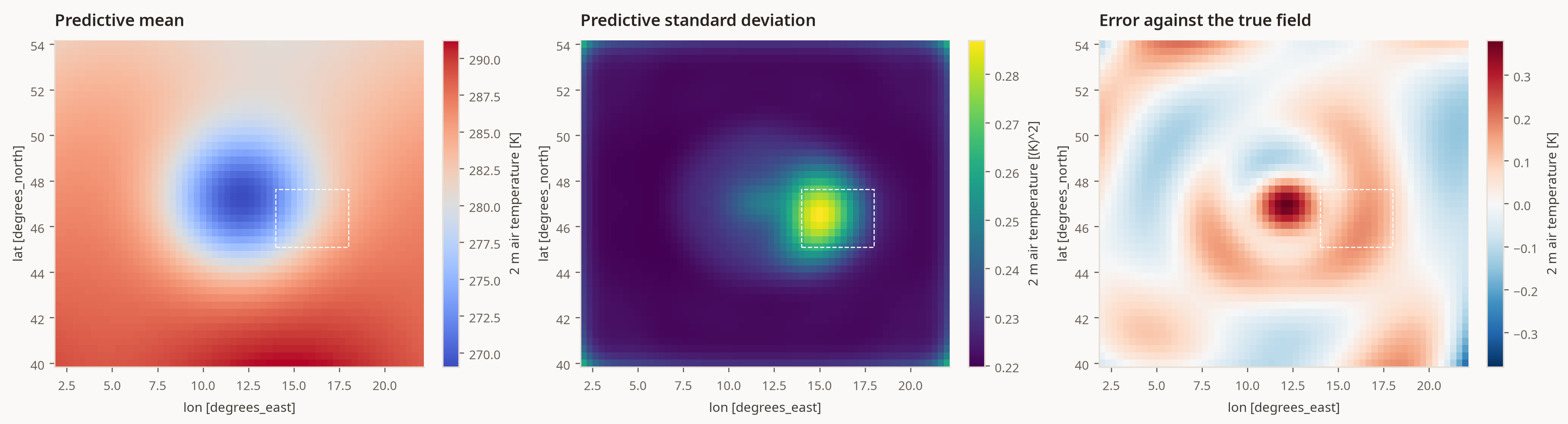
The standard deviation grows inside the dashed box where observations were missing, and the error stays small across the mountain range because elevation is an input.
Joint samples and regional averages#
The mean and variance describe each cell on its own. Many questions are about several cells together, such as the average temperature over the Alpine box \(\mathcal{R}\). Its variance depends on the covariance between the cells,
which the per-cell variances alone cannot give. For this we need the full
covariance, so we build all the prediction inputs at once with
spec.inputs_for. Passing num_samples to to_xarray then draws from the joint
predictive distribution, and returns the draws with a leading sample
dimension. Averaging each draw over the region gives samples of the regional
mean.
test_inputs, test_spec = spec.inputs_for(fine[["elevation"]])
latent = posterior(test_inputs)  # the field itself, without observation noise
key, sample_key = jr.split(key)
samples = test_spec.to_xarray(latent, num_samples=500, key=sample_key)

alps = dict(lat=slice(45.0, 49.0), lon=slice(8.0, 16.0))
regional_mean = samples["t2m"].sel(**alps).mean(["lat", "lon"])
true_regional_mean = float(fine["t2m"].sel(**alps).mean())

# The same latent distribution, but treating the cells as independent.
latent_variance = test_spec.to_xarray(latent)["t2m_variance"].sel(**alps)
joint_std = float(regional_mean.std("sample"))
naive_std = float(np.sqrt(latent_variance.sum()) / latent_variance.size)

print(f"Regional mean: {float(regional_mean.mean()):.2f} K (truth {true_regional_mean:.2f} K)")
print(f"Standard deviation from joint samples:        {joint_std:.3f} K")
print(f"Standard deviation if cells were independent: {naive_std:.3f} K")
Regional mean: 275.11 K (truth 275.03 K)
Standard deviation from joint samples:        0.065 K
Standard deviation if cells were independent: 0.007 K
Treating the cells as independent understates the uncertainty in the regional
average by roughly an order of magnitude, because neighbouring cells tend to be
wrong in the same direction. Against the joint standard deviation the true
regional mean is a plausible outcome; against the independent one it would look
like a many-sigma surprise. Joint
samples keep that correlation, which is why to_xarray refuses to draw samples
from a distribution that only holds marginal variances (as returned by
posterior(test_inputs, covariance="diagonal")).
Global grids and seasonal cycles#
Latitude and longitude in degrees are not good inputs for a global field. A
degree of longitude is about 111 km at the equator but only 38 km at 70°N, and
longitude 359° is next to 0°. The
UnitSphere transform replaces lat and lon with
the three coordinates of a point on the unit sphere. A stationary kernel on these
coordinates uses the chord distance through the Earth, which has no seam and no
distortion at the poles. In the same way, Cyclic
encodes a periodic input as a point on a circle. Datetime inputs are days since
their first timestamp, so a period of 365.25 gives the seasonal cycle:
data, spec = from_xarray(
    ds,
    target="t2m",
    inputs=["lat", "lon", "time", "elevation"],
    transforms=[UnitSphere(), Cyclic("time", 365.25), Standardise(["elevation"])],
)
spec.columns
# ('sphere_x', 'sphere_y', 'sphere_z', 'time_sin', 'time_cos', 'elevation')
The transforms run in order, and spec.columns names the columns of
\(\mathbf{X}\) that they produce, one for each kernel lengthscale.
Infilling Global Surface Temperature uses
UnitSphere on a real global field.
System configuration#
%reload_ext watermark
%watermark -n -u -v -iv -w -a 'Thomas Pinder'
Author: Thomas Pinder

Last updated: Sun, 04 Oct 2026

Python implementation: CPython
Python version       : 3.11.16
IPython version      : 9.17.1

gpjax     : 1.0.0
jax       : 0.10.2
jaxtyping : 0.3.11
logging   : 0.5.1.2
matplotlib: 3.11.2
numpy     : 2.4.6
xarray    : 2026.7.0

Watermark: 2.6.0