Infilling Global Surface Temperature#
Download this notebook: infilling_surface_temperature.ipynb
Temperature records have gaps: over the poles, over parts of Africa and the Southern Ocean, and, for satellites, wherever there is cloud. Climate scientists fill these gaps to map the field and to compute the global mean temperature. In this notebook we fill gaps with a GP, and we test the result.
To know how good the filled values are, we start from a field that is complete, remove cells ourselves, and compare the GP with the cells that we removed. We
fill gaps that are random, map the field, and get the global mean temperature with its uncertainty from joint posterior samples, and
show what goes wrong when cells are missing because of their values.
The notebook uses the gpjax.xarray module, which
Working with Gridded Data introduces. It needs the
optional extra: pip install "gpjax[xarray]".
from pathlib import Path

from jax import config
import jax.numpy as jnp
import jax.random as jr
from jaxtyping import install_import_hook
import matplotlib.pyplot as plt
import numpy as np
import xarray as xr

config.update("jax_enable_x64", True)

with install_import_hook("gpjax", "beartype.beartype"):
    import gpjax as gpx
    from gpjax.parameters import val
    from gpjax.xarray import (
        UnitSphere,
        from_xarray,
    )

key = jr.key(42)
rng = np.random.default_rng(0)
gpx.plotting.use_style()
'ledger'
A complete temperature field#
We use the NCEP-NCAR Reanalysis 1 (Kalnay et al., 1996). A reanalysis combines a weather model with the observations, so it has a value in every grid cell. The file holds the 2024 annual-mean near-surface air temperature as an anomaly: the difference from the 1991–2020 mean of the same cell. Anomalies remove the large, fixed differences between the equator and the poles, so what remains is the signal of interest, and it varies smoothly over large distances.
NCEP-NCAR Reanalysis 1 data provided by the NOAA PSL, Boulder, Colorado, USA, from their website at https://psl.noaa.gov.
nc_candidates = [
    Path("docs/examples/data/ncep_air_anomaly_2024.nc"),
    Path("data/ncep_air_anomaly_2024.nc"),
]
nc_path = next(path for path in nc_candidates if path.exists())
reanalysis = xr.open_dataset(nc_path)
reanalysis
<xarray.Dataset> Size: 43kB
Dimensions:      (lat: 73, lon: 144)
Coordinates:
  * lat          (lat) float32 292B -90.0 -87.5 -85.0 -82.5 ... 85.0 87.5 90.0
  * lon          (lon) float32 576B -180.0 -177.5 -175.0 ... 172.5 175.0 177.5
Data variables:
    tas_anomaly  (lat, lon) float32 42kB ...
Attributes:
    title:            2024 annual-mean near-surface air temperature anomaly
    source:           NCEP-NCAR Reanalysis 1, monthly air.sig995 (air.mon.mea...
    references:       Kalnay et al. (1996), doi:10.1175/1520-0477(1996)077<04...
    acknowledgement:  NCEP-NCAR Reanalysis 1 data provided by the NOAA PSL, B...
    history:          Annual means of the monthly means; 2024 minus the 1991-...
Conventions: CF-1.8The native grid is 2.5°. We fit on a 5° grid, which is every second grid point, and predict back on the 2.5° grid, so the predictions are also tested at points the model never saw.
truth_fine = reanalysis["tas_anomaly"].astype(float)
truth = truth_fine.isel(lat=slice(1, None, 2), lon=slice(1, None, 2))
print(f"5° grid: {dict(truth.sizes)}, 2.5° grid: {dict(truth_fine.sizes)}")

anomaly_style = dict(cmap="RdBu_r", vmin=-4.0, vmax=4.0)
error_style = dict(
    cmap="PuOr_r", vmin=-2.0, vmax=2.0, cbar_kwargs={"label": "Error [K]"}
)
truth_fine.plot(figsize=(7, 3.5), **anomaly_style)
plt.title("2024 anomaly, NCEP-NCAR Reanalysis 1")
plt.show()
5° grid: {'lat': 36, 'lon': 72}, 2.5° grid: {'lat': 73, 'lon': 144}
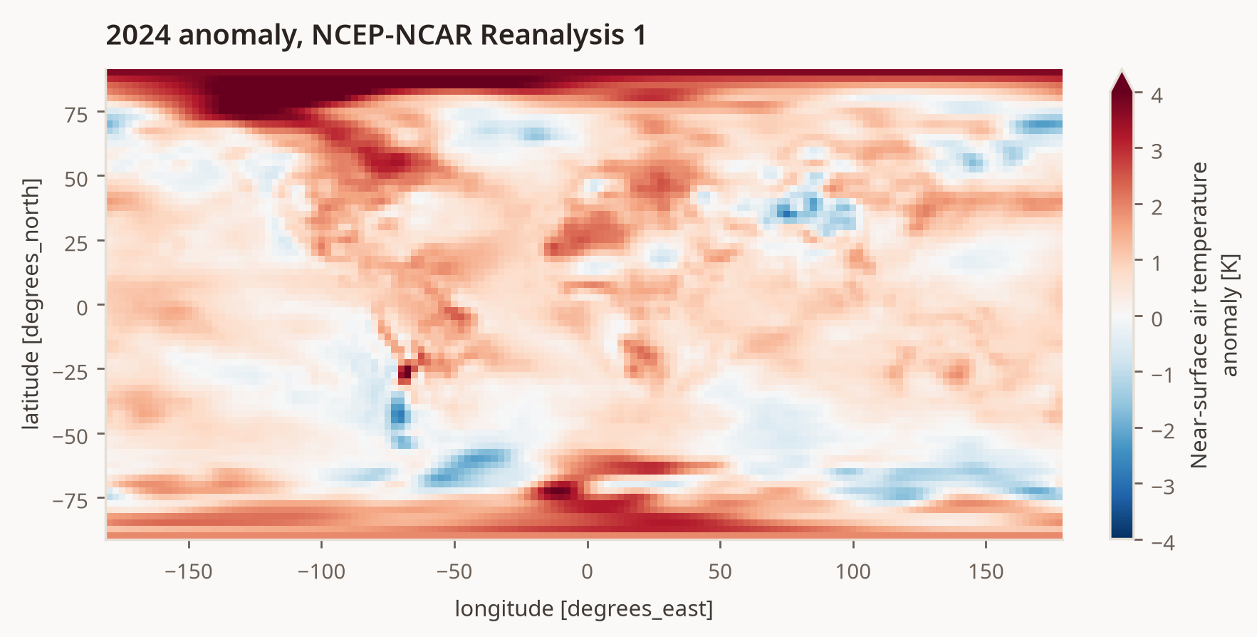
A 5° cell near a pole is much smaller than one at the equator, so a global mean weights each cell by the cosine of its latitude.
True global mean anomaly: 0.64 K
Cells missing at random#
First we keep a random 25% of the 5° cells. Which cells are missing has nothing to do with their values. Statisticians call this missing completely at random.
664 of 2592 cells kept
Inputs on the sphere#
Latitude and longitude in degrees are not good GP inputs for a global field. A
5° cell is about 555 km wide at the equator but only about 24 km wide next to a
pole, and longitude 177.5°E is next to 177.5°W. The
UnitSphere transform replaces lat and lon with
the three coordinates of a point on the unit sphere. A stationary kernel on these
coordinates uses the chord distance through the Earth, so it has no seam at the
antimeridian and no distortion at the poles. Its lengthscale is in Earth radii.
Dataset(Number of observations: 664 - Input dimension: 3)
GridSpec(target='tas', inputs=('lat', 'lon'), columns=('sphere_x', 'sphere_y', 'sphere_z'), grid={'lat': 36, 'lon': 72}, kept=664, dropped=1928)
Fitting the model#
We use a Matérn-3/2 kernel, which gives rougher fields than an RBF kernel, as temperature anomalies are. A constant mean absorbs the global warming signal.
def fit_model(train_data: gpx.Dataset):
    prior = gpx.gps.Prior(
        mean_function=gpx.mean_functions.Constant(jnp.array([0.5])),
        kernel=gpx.kernels.Matern32(lengthscale=jnp.array(0.3), variance=1.0),
    )
    model = prior * gpx.likelihoods.Gaussian(obs_stddev=jnp.array(0.1))
    model, _ = gpx.fit_scipy(
        model=model,
        objective=lambda candidate, train_data: (
            -gpx.objectives.conjugate_mll(candidate, train_data)
        ),
        train_data=train_data,
        verbose=False,
    )
    return model


earth_radius_km = 6371.0
model = fit_model(data)
lengthscale_km = float(val(model.prior.kernel.lengthscale)) * earth_radius_km
print(f"Lengthscale: {lengthscale_km:.0f} km")
Lengthscale: 798 km
Predicting on the finer grid#
spec.predict gives the predictive mean and variance on the 2.5° grid of the
reanalysis, in chunks of chunk_size cells. We use a diagonal covariance,
because we need only the variance of each cell.
posterior = model.condition(data)
prediction = spec.predict(
    lambda x: model.likelihood(posterior(x, covariance="diagonal")),
    truth_fine.to_dataset(),
    chunk_size=2048,
)
prediction
<xarray.Dataset> Size: 169kB
Dimensions:       (lat: 73, lon: 144)
Coordinates:
  * lat           (lat) float32 292B -90.0 -87.5 -85.0 -82.5 ... 85.0 87.5 90.0
  * lon           (lon) float32 576B -180.0 -177.5 -175.0 ... 172.5 175.0 177.5
Data variables:
    tas_mean      (lat, lon) float64 84kB 1.978 1.978 1.978 ... 3.677 3.677
tas_variance (lat, lon) float64 84kB 0.02097 0.02097 ... 0.02059 0.02059Because the field is complete, we can score every prediction. We compare with a simple baseline, the mean of the kept cells, and check the uncertainty: about 95% of the true values should be within two predictive standard deviations.
def score(prediction: xr.Dataset, observed: xr.Dataset) -> None:
    error = prediction["tas_mean"] - truth_fine
    baseline_error = float(observed["tas"].mean()) - truth_fine
    within = abs(error) < 2 * np.sqrt(prediction["tas_variance"])
    print(f"RMSE, GP:                {float(np.sqrt((error**2).mean())):.2f} K")
    print(
        f"RMSE, mean of kept cells: {float(np.sqrt((baseline_error**2).mean())):.2f} K"
    )
    print(f"Within 2 sd:             {float(within.mean()):.0%}")


def plot_infill(prediction: xr.Dataset, observed: xr.Dataset) -> None:
    fig, axes = plt.subplots(1, 3, figsize=(15, 3.5), sharey=True)
    observed["tas"].plot(ax=axes[0], **anomaly_style)
    axes[0].set_title("Kept cells")
    prediction["tas_mean"].plot(ax=axes[1], **anomaly_style)
    axes[1].set_title("Predictive mean")
    (prediction["tas_mean"] - truth_fine).plot(ax=axes[2], **error_style)
    axes[2].set_title("Predictive mean minus truth")
    for ax in axes[1:]:
        ax.set_ylabel("")
    plt.show()


score(prediction, observed)
plot_infill(prediction, observed)
RMSE, GP:                0.33 K
RMSE, mean of kept cells: 1.05 K
Within 2 sd:             94%
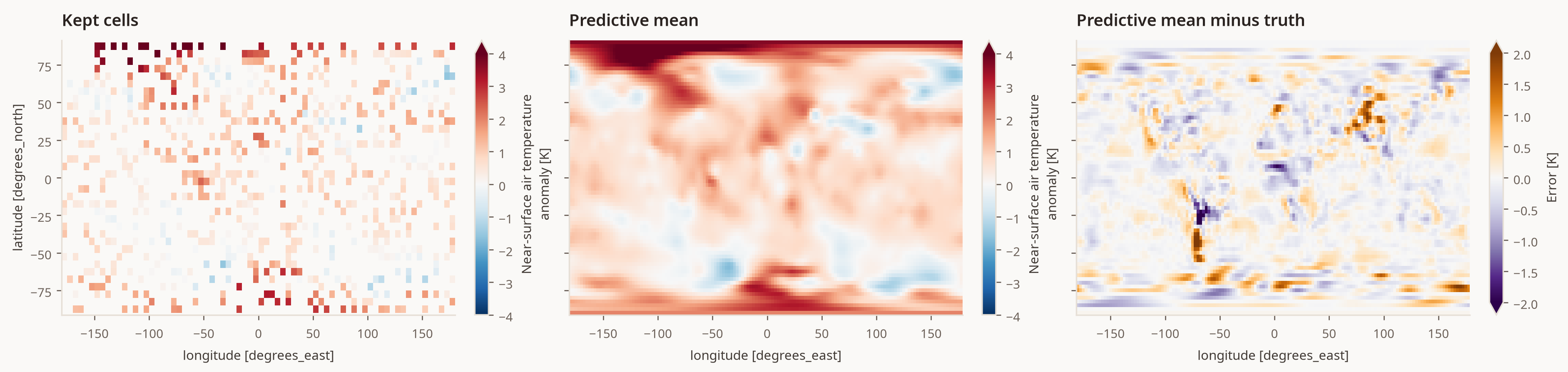
From a quarter of the cells, the GP recovers the large-scale pattern, including the strong warmth over the Arctic. The errors are largest where the field changes over short distances, and the uncertainty is about right.
The global mean, with joint samples#
The global mean anomaly fills each missing cell and averages. Its variance depends on the covariance between the filled cells,
which the per-cell variances alone cannot give. For this we need the full
covariance, so we build all the prediction inputs on the 5° grid at once with
spec.inputs_for. Passing num_samples to to_xarray then draws from the joint
distribution of the field, and returns the draws with a leading sample
dimension. combine_first keeps the kept cells and takes each missing cell from
a draw.
def global_mean_samples(posterior, spec, observed: xr.Dataset, key) -> xr.DataArray:
    test_inputs, test_spec = spec.inputs_for(truth.to_dataset())
    samples = test_spec.to_xarray(posterior(test_inputs), num_samples=500, key=key)
    return global_mean(observed["tas"].combine_first(samples["tas"]))


def report_global_mean(means: xr.DataArray, observed: xr.Dataset) -> None:
    print(f"Truth:               {float(global_mean(truth)):.2f} K")
    print(f"Mean of kept cells:  {float(global_mean(observed['tas'])):.2f} K")
    print(
        f"Gaps filled by GP:   {float(means.mean()):.2f}"
        f" ± {2 * float(means.std('sample')):.2f} K (2 sd)"
    )


key, sample_key = jr.split(key)
means = global_mean_samples(posterior, spec, observed, sample_key)
report_global_mean(means, observed)
Truth:               0.64 K
Mean of kept cells:  0.65 K
Gaps filled by GP:   0.63 ± 0.04 K (2 sd)
With random gaps, even the mean of the kept cells is close to the truth, and the GP gives the global mean with an interval that holds it.
Cells missing because of their values#
Real gaps are rarely random. A satellite cannot see the surface through cloud, a station fails in extreme weather, and the polar regions, which warm fastest, have the fewest observations. When the chance that a cell is missing depends on the value that is missing, the data are missing not at random.
We simulate this. We again aim to keep a quarter of the cells, but now the warmer a cell’s anomaly, the less likely it is to be kept.
standardised = ((truth - truth.mean()) / truth.std()).values
odds = np.exp(-1.5 * standardised)
keep_probability = np.clip(0.25 * odds / odds.mean(), 0.0, 1.0)
kept_selectively = rng.uniform(size=truth.shape) < keep_probability
selective = truth.where(kept_selectively).rename("tas").to_dataset()
print(f"{int(kept_selectively.sum())} of {truth.size} cells kept")
534 of 2592 cells kept
The steps are the same as before.
data_selective, spec_selective = from_xarray(
    selective, target="tas", inputs=["lat", "lon"], transforms=[UnitSphere()]
)
model_selective = fit_model(data_selective)
posterior_selective = model_selective.condition(data_selective)
prediction_selective = spec_selective.predict(
    lambda x: model_selective.likelihood(posterior_selective(x, covariance="diagonal")),
    truth_fine.to_dataset(),
    chunk_size=2048,
)

score(prediction_selective, selective)
plot_infill(prediction_selective, selective)

key, sample_key = jr.split(key)
means_selective = global_mean_samples(
    posterior_selective, spec_selective, selective, sample_key
)
report_global_mean(means_selective, selective)
RMSE, GP:                0.97 K
RMSE, mean of kept cells: 1.37 K
Within 2 sd:             81%
Truth:               0.64 K
Mean of kept cells:  0.06 K
Gaps filled by GP:   0.34 ± 0.05 K (2 sd)
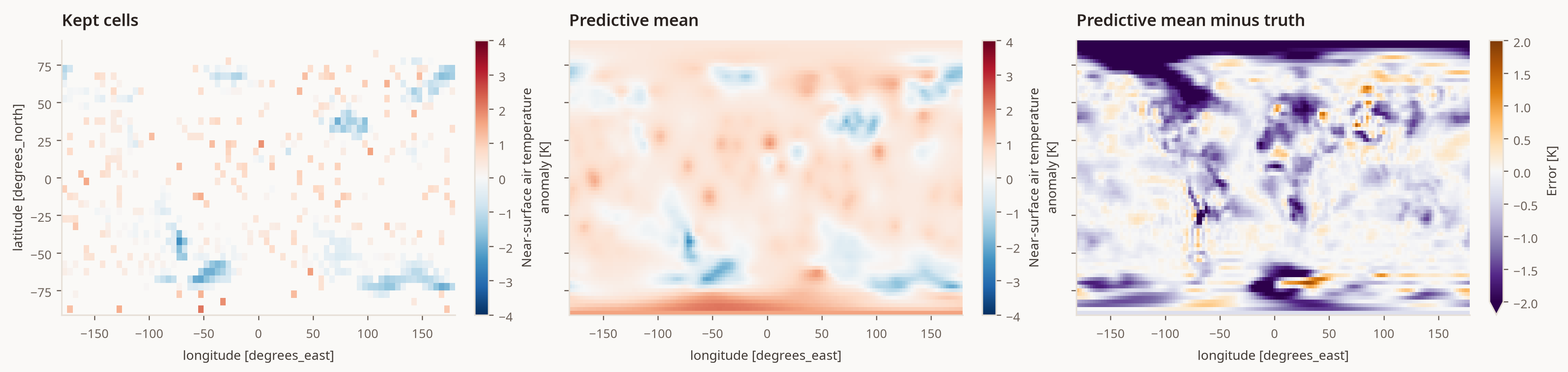
The kept cells are mostly the cold ones, so their mean is far too cold. The GP removes part of this bias, because it fills each gap from its neighbours and the warm regions still have some kept cells. But the result is still too cold, and the interval does not hold the truth: the GP is confidently wrong.
The reason is that a GP conditions only on the values it sees. Its prior has one constant mean, which it learns from the kept cells, so the cold kept cells pull that mean down. It also has no way to know that the missing cells are warm, because nothing in its inputs says so. Its uncertainty describes the spread of values that are consistent with the kept cells, not the error of the selection.
In real data we cannot see this bias, because we do not have the missing values. Useful steps are:
Add inputs that explain why cells are missing, such as cloud fraction or a covariate that is observed everywhere. If the chance of a gap depends only on the inputs, the gaps are missing at random given those inputs, and the GP can correct for them.
Model the observation process together with the field.
Test how sensitive the result is to different assumptions about the missing values, as we did here with a complete field.
Adding an input that explains the gaps#
If a variable that explains the gaps is observed everywhere, add it as an input.
Standardise puts it on the same scale as the
sphere coordinates:
data, spec = from_xarray(
    observed,
    target="tas",
    inputs=["lat", "lon", "cloud_fraction"],
    transforms=[UnitSphere(), Standardise(["cloud_fraction"])],
)
For a monthly record, Cyclic adds the seasonal cycle;
see Working with Gridded Data.
References#
Kalnay, E., Kanamitsu, M., Kistler, R., Collins, W., Deaven, D., Gandin, L., Iredell, M., Saha, S., White, G., Woollen, J., Zhu, Y., Chelliah, M., Ebisuzaki, W., Higgins, W., Janowiak, J., Mo, K. C., Ropelewski, C., Wang, J., Leetmaa, A., Reynolds, R., Jenne, R. and Joseph, D. (1996). The NCEP/NCAR 40-year reanalysis project. Bulletin of the American Meteorological Society, 77(3), 437–471. doi:10.1175/1520-0477(1996)077<0437:TNYRP>2.0.CO;2
System configuration#
%reload_ext watermark
%watermark -n -u -v -iv -w -a 'Thomas Pinder'
Author: Thomas Pinder

Last updated: Sun, 04 Oct 2026

Python implementation: CPython
Python version       : 3.11.16
IPython version      : 9.17.1

gpjax     : 1.0.0
jax       : 0.10.2
jaxtyping : 0.3.11
logging   : 0.5.1.2
matplotlib: 3.11.2
numpy     : 2.4.6
xarray    : 2026.7.0

Watermark: 2.6.0